Trade-Adjusted Scope 3 Emissions: Why Purchase Location Can Misrepresent the Supply Chain

A company buys a computer in Malaysia. The finance system records a Malaysian supplier, a Malaysian invoice and an amount in ringgit, and the purchase is coded to electronics. For a spend-based Scope 3 calculation, that is often all the information there is.

Ask where the computer was made and the answer is rarely Malaysia alone. Its processor may have been fabricated in Taiwan, its memory and display made in two other countries and the whole machine assembled in a fourth before it was shipped to a distributor. The invoice records the last step of that chain. It says nothing about the steps before it.

The same is true of servers, networking equipment, CCTV systems, machinery, industrial and electrical equipment, vehicles and office equipment. In each case the place of purchase and the place of production are different facts, and a Scope 3 calculation has to decide which of them its emission factor represents.

Country-specific factors are useful, but incomplete

Country-specific emission factors exist for good reasons. Economies differ in their electricity systems, energy mix, industrial profile, production structure and prices. A factor built for the Malaysian economy reflects some of that. It is usually more representative than a single global average applied to every transaction.

The difficulty lies in the level at which it operates. A purchase coded to electronics in Malaysia may receive a factor describing Malaysian expenditure on electronic equipment. That factor has not necessarily identified where the semiconductors were made, where the memory or display was produced, where assembly took place, how far the components travelled or which countries supplied the intermediate goods. How much of this a given factor captures depends on how it was built. Some single-country models assume that imported goods were produced with the same technology and energy mix as domestic ones; others treat imports more explicitly. Either way, one country-level number stands in for a production geography it does not show.

The first article in this series, on spend-based Scope 3 emissions, argued that the emission factor is only the starting point: currency, price year and the meaning of the expenditure all have to be settled before the multiplication means anything. It left one question open for later. A factor can be in the right currency and the right price year and still describe the wrong place.

Malaysia and the UK

Now place a similar computer on a UK invoice. It will probably be assigned a UK electronics factor, while the Malaysian purchase receives a Malaysian one, and the two factors may differ considerably. Yet the two computers may contain substantially similar components from the same international manufacturing network.

Two companies can buy the same broad category of product in different countries while drawing on largely the same global supply chain.

It does not follow that the two footprints are the same, nor that either country should have the lower figure. Assembly may take place in different locations for different markets. Transport routes and distribution networks differ by destination. The electricity intensity of manufacturing differs between the countries where production actually happens, and each country-level factor may represent imports and economic relationships in its own way. The result depends on the supply chain and on the method, which is precisely the point.

“Electronics” is not one product

The category does some obscuring of its own. A ledger line for computers and electronic equipment can cover all of these:

• Laptops
• Servers
• Memory modules
• Semiconductors
• CCTV cameras
• Network switches
• Monitors
• Storage equipment
• Sensors
• Telecommunications equipment

They differ in production process, energy demand, material composition, supplier network, manufacturing country, assembly location and trade route. A factor can therefore be country-specific and still broad in product terms; a single electronics factor may represent some of these purchases far better than others.

The third article in this series, on custom emission factors, reached a similar conclusion about suppliers: being specific in one dimension does not guarantee that a number represents the purchase. A supplier factor built from the supplier’s own Scope 1 and Scope 2 describes one tier of the chain. The components it buys in were made upstream, in whichever countries made them, and their emissions sit outside the supplier’s inventory altogether.

The trade layer

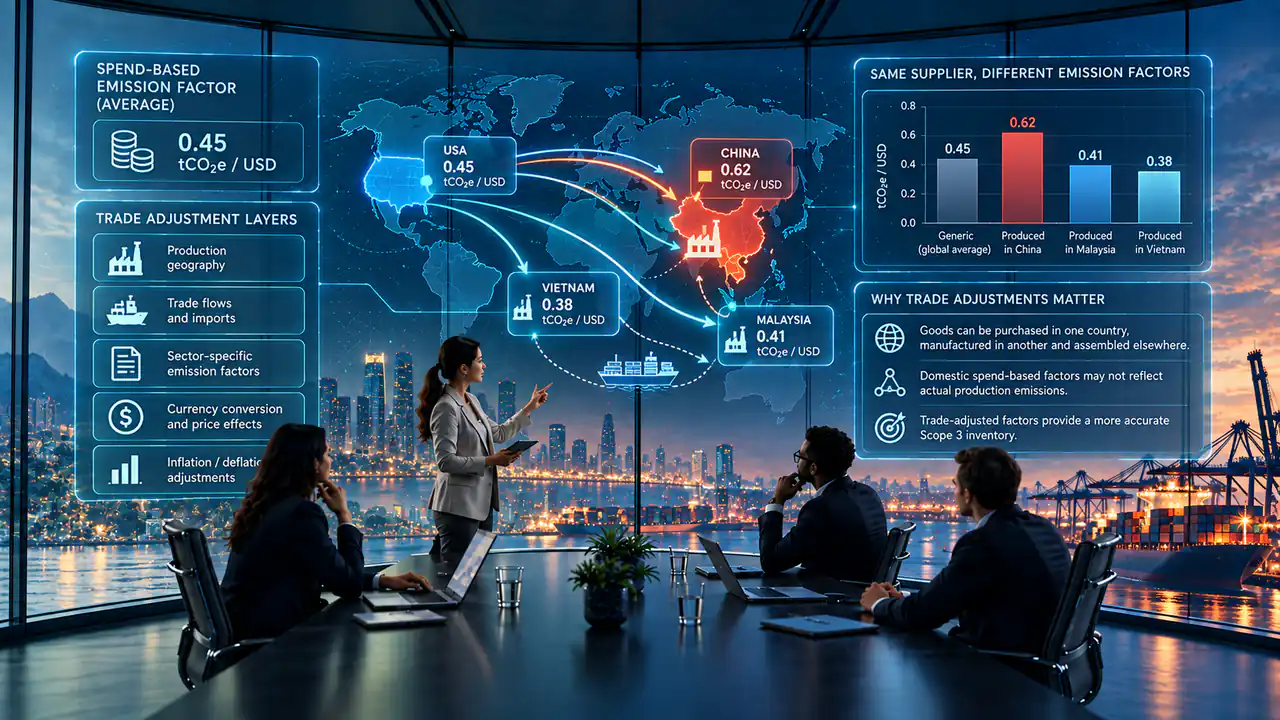
A trade-adjustment layer brings into the calculation information that a purchasing-country factor does not carry: the countries a product and its inputs come from, the trade relationships between exporting and importing economies, the product or industry classification, the intermediate inputs that pass between industries and where the underlying production takes place.

The objective is not to establish the exact carbon footprint of each individual product. It is to make the emission factor more representative of the economic and geographical structure behind the purchase.

Supply chains have more than one border

A trade layer would be simple if every import had one origin. It rarely does. A computer bought in Malaysia is not just a Malaysian purchase of a product from one other country: raw materials are extracted in one place, components manufactured in another, processed in a third and assembled in a fourth before the product is distributed to the buyer.

Each stage can happen in a different country, on a different energy system, with its own suppliers. By the time of the final purchase, the product may contain economic activity from several countries, some of which the importer has never traded with directly.

Where input-output and trade models come in

Representing a chain like that requires a model of how economies supply one another. Multi-regional input-output (MRIO) models link national tables of industry inputs and outputs through bilateral trade, so that the intermediate goods one country’s industries buy from another’s can be traced through to final demand. Combined with emissions data for each industry in each country, they can estimate the emissions embodied in traded goods and services, together with the economies in which those emissions arose.

The same family of models underpins the comparison between production-based national inventories and consumption-based footprints, which attribute emissions to the economies whose final demand drives them rather than those where they physically occur. A company’s Scope 3 calculation borrows the machinery for a narrower purpose: describing the upstream emissions of what it bought.

What such a model produces is a modelled representation of international economic relationships, built from trade statistics, national accounts and a set of assumptions. It is not a measured product footprint. It describes average relationships between industries and countries, which is why it can make a spend-based calculation more representative of geography without making it exact.

A practical extension of the GHG Protocol

The GHG Protocol’s Category 1 guidance describes four methods for purchased goods and services: supplier-specific, hybrid, average-data and spend-based. The hybrid method combines supplier-specific activity data with secondary data to fill the gaps, on the recognition that one source rarely describes a purchase completely. The Scope 3 Standard, for its part, lists geographical representativeness among its data quality indicators: the degree to which the data reflects the actual location of the activity.

Neither document calls for a trade-adjustment layer by name. Accounting for international trade is better understood as a practical extension of the principle both rest on: the calculation method should be appropriate to the activity being represented, and for an imported good much of that activity took place somewhere else.

Why this becomes difficult at scale

A company may have tens of thousands of purchases across hundreds of suppliers, in several currencies, under many product classifications and from many countries of origin. Working out the trade structure behind each transaction by hand in a spreadsheet stops being practical long before the end of the ledger.

The question also changes shape. It is no longer amount multiplied by factor. It becomes what was bought, where it came from, what economic activity it represents and which trade relationships sit behind it.

That is the transaction-level work the earlier articles described. Imported goods add routes of their own to the problem set out in the second, on Scope 3 double counting: freight, customs brokerage and logistics charges are often invoiced separately from the goods, and each needs a clear rule about which calculation it belongs to before any factor, trade-adjusted or not, is applied.

The practical question

If the purchase is recorded in Malaysia, should the whole calculation rest on a Malaysian factor? There is no blanket answer. It depends on what the factor represents and whether it adequately captures the economic and geographical character of the good or service purchased. For services delivered locally a country factor may be entirely appropriate.

A trade-adjusted approach adds most where international supply chains are significant: where imported goods make up a large share of expenditure, where product categories involve complex global manufacturing and where the country-level factor is too broad for the purchase. It earns its cost where the company needs a more representative inventory for decisions or disclosure and where transaction volumes justify the extra modelling.

A trade-adjusted model still rests on sector averages, trade statistics, country-level production data and estimated shares of origin. What it offers is a more representative model of the activity behind the purchase than one that assumes the purchasing country did all the producing. Moving a category onto that basis is also a change in methodology. Where its effect is significant, the comparative year may need to follow, which is the subject of the final article in this series, on restating GHG emissions.

Where the activity happened

The country on the invoice is an accounting fact. It is not necessarily a description of the supply chain.

A robust spend-based Scope 3 calculation therefore requires more than an emission factor. It may require an understanding of the transaction, the product, the countries involved and the economic relationships that connect them.

Ace CSR supports Malaysian companies with Scope 3 assessment, GHG accounting and sustainability reporting, including the classification of purchases, the choice of factor for imported goods and the methodology notes that explain it.

References

- GHG Protocol, Technical Guidance for Calculating Scope 3 Emissions, Category 1, on the supplier-specific, hybrid, average-data and spend-based methods and the use of secondary data to fill gaps in supplier data.
- GHG Protocol, Corporate Value Chain (Scope 3) Accounting and Reporting Standard, Chapter 7, on the data quality indicators, including geographical representativeness.
- Wiedmann, T., ‘A review of recent multi-region input–output models used for consumption-based emission and resource accounting’, Ecological Economics 69(2), 2009, pp. 211–222.
- Peters, G. P. and Hertwich, E. G., ‘CO2 embodied in international trade with implications for global climate policy’, Environmental Science & Technology 42(5), 2008, pp. 1401–1407.