
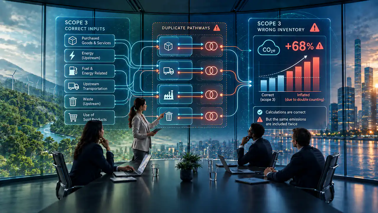
GHG Emissions · Part 2 of 3
Scope 3 Double Counting: When Correct Calculations Produce the Wrong Inventory
Most checks on a Scope 3 figure are checks on a calculation. Was the right factor chosen, were the units converted properly, does the multiplication hold? Those questions matter, and an inventory can pass every one of them and still be wrong.
Take three calculations any reviewer would accept on sight: expenditure multiplied by a spend-based factor, kilometres multiplied by a transport factor and tonnes of waste multiplied by a treatment factor. Each is technically correct. If two of them describe the same underlying activity, the inventory that adds them together is not. RM500,000 of logistics expenditure multiplied by an appropriate factor is a sound calculation; if the same shipments have already been calculated from their weights and distances, adding the spend-based result counts the freight twice, and nothing in either calculation will reveal it.
That is the distinction this article is about. A correct calculation is a property of a formula. A correct inventory is a property of how the data behind every formula fits together, and the two can come apart without anyone having made a mistake.
At a Glance
One Activity, Two Correct Calculations
A Year of Inbound Freight
HypotheticalUnderlying Activity
The same shipments, moved once
Activity-based route
Shipment records
tonnes × kilometres × transport factor
310 tCO2e
Correct calculation
Spend-based route
Logistics expenditure, RM 500,000
expenditure × spend-based factor
265 tCO2e
Correct calculation
Inventory as reported
575 tCO2e
Overstated by roughly 85%, with no error in either calculation to find.
correct calculation + duplicated activity = incorrect inventory
Hypothetical figures, not client data. The shorthand above is an explanation, not a GHG Protocol equation. The problem may not be the calculation; it may be that the underlying activity has been represented twice.
Three kinds of double counting; only one is the problem here
Double counting is a loose term, and it covers situations the GHG Protocol treats very differently. Three are worth separating before going any further.
Inherent
Across companies
One company’s Scope 1 is its customers’ Scope 3. The same value-chain emissions legitimately appear in several inventories; that is how value-chain accounting works.
Prevented by definition
Between scopes
The scopes are defined so a company’s own emissions sit in one of them. Scope 3 covers the indirect emissions that Scopes 1 and 2 do not.
This article
Within one Scope 3 inventory
The categories are designed to be mutually exclusive. The datasets feeding them are not, and one activity can arrive by several routes.
The first is not an error. The Corporate Standard defines Scopes 1 and 2 so that two companies do not account for the same emissions in the same scope, while accepting that one company’s Scope 1 can be another’s Scope 2. Scope 3 extends the same logic along the value chain: a supplier’s direct emissions are, quite properly, part of its customers’ Scope 3. Nobody should try to engineer that overlap out of their inventory.
The second and third are different, because both happen inside a single company’s report. The Scope 3 calculation guidance states that the fifteen categories are designed to be mutually exclusive to avoid a company double counting emissions among categories, and it defines Category 1 as purchased goods and services not otherwise included in Categories 2 to 8.
The categories, in other words, are clean. The data arriving at them is not organised by category, and one economic activity can reach the inventory through a spend-based calculation, an activity-based one, a second category, a separate operational dataset or a transaction between two companies in the same group. That is the practical problem, and it is the subject of the rest of this article.
The financial ledger is not an emissions inventory
The first article in this series, on spend-based Scope 3 emissions, argued that a spend-based calculation involves far more than expenditure multiplied by a factor: currency, price year and sector classification all have to be settled before the multiplication means anything. This article starts one step earlier, with what the expenditure represents.
Financial data is attractive for Scope 3 because it is complete. Almost everything a company buys passes through the general ledger, so a spend-based calculation offers coverage that no other dataset can match. The ledger, however, was built to record financial obligations rather than physical activity, and many of the activities it records in ringgit are also recorded somewhere else, in litres, kilowatt-hours, tonnes or kilometres.
Two Records of One Activity
What the Ledger Also Records Somewhere Else
Underlying activity
In the ledger
Elsewhere, in physical units
Usually reported in
Fuel
In the ledger
Fuel expenditure
Elsewhere, in physical units
Litres by fuel type
Usually reported in
Electricity
In the ledger
Electricity bills
Elsewhere, in physical units
kWh by site and grid
Usually reported in
Waste
In the ledger
Waste contractor invoices
Elsewhere, in physical units
Tonnes by waste type and treatment route
Usually reported in
Freight
In the ledger
Logistics expenditure
Elsewhere, in physical units
Tonnes, distance and mode, or tonne-km
Usually reported in
Business travel
In the ledger
Travel and expense accounts
Elsewhere, in physical units
Passenger-km by mode and class
Usually reported in
Every row is one activity recorded twice. Run the ledger column through spend-based factors and the right-hand column through activity-based ones, and each activity can enter the inventory by both routes.
Category placement shows the common case. It depends on the organisational boundary and on who paid for the activity: freight paid for by a supplier, for example, is not reported in Category 4 by the buyer.
None of this means every such line must be removed from a spend-based calculation under every methodology. Where no activity data exists, the expenditure may be the best representation of an activity there is. The claim is narrower than that.
The financial ledger can provide the starting point for a spend-based calculation, but it cannot automatically be treated as a separate source of emissions.
Fuel and electricity: the obvious overlaps
Fuel is the clearest case. A company running a fleet or standby generators calculates Scope 1 from litres of diesel multiplied by a combustion factor and will usually calculate the upstream emissions of producing and delivering that diesel in Category 3, which the Scope 3 Standard names fuel- and energy-related activities not included in Scope 1 or Scope 2. The same diesel appears in the ledger as fuel expenditure. Run the whole ledger through spend-based factors and that expenditure acquires a second estimate.
Where the second estimate overlaps depends on what the spend factor covers, and it is easy to miss. An input-output factor for refined petroleum products describes the emissions of producing the fuel, not of burning it, so the overlap is chiefly with the upstream emissions already in Category 3. A spend factor that includes combustion overlaps with Scope 1 directly. Either way the diesel has been represented twice, and which part is duplicated is answered by the factor’s documentation rather than by the ledger.
Electricity follows the same logic with a sharper edge. Scope 2 is kilowatt-hours multiplied by a grid emission factor, with upstream and transmission-related emissions in Category 3. An input-output factor for the electricity sector is dominated by the emissions of generating electricity, which are precisely what Scope 2 already reports. Applied to the electricity bill, it counts the same generation a second time.
The Obvious Overlaps
One Purchase, Two Routes into the Inventory
One Purchase
Diesel for a fleet or generators
Physical Record
Litres
litres × combustion factor
Scope 1litres × upstream fuel factor
Category 3
Financial Record
Fuel expenditure
RM × spend-based factor
Category 1, if not filteredWhere the Overlap Falls
A cradle-to-gate spend factor repeats the upstream emissions already in Category 3. A factor that includes combustion repeats Scope 1 as well. The factor’s documentation, not the ledger, says which.
One Purchase
Electricity for offices and sites
Physical Record
kWh
kWh × grid emission factor
Scope 2kWh × upstream and T&D factors
Category 3
Financial Record
Electricity bills
RM × electricity-sector factor
Category 1, if not filteredWhere the Overlap Falls
An input-output factor for the electricity sector is dominated by the emissions of generating it: the same generation Scope 2 already reports.
Illustrative. A utility or fuel account can also carry items the physical record does not cover, such as connection charges, equipment or lubricants, which is why the boundary has to be settled before any exclusion is applied.
The response is not to delete every fuel and electricity line from Category 1 by reflex. A utility account can include connection charges, equipment and services that sit outside the kilowatt-hours; a fuel account can hold lubricants alongside diesel. The reporting boundary and the calculation methodology have to be established first. Only then is it clear which part of a transaction is already captured and which is not.
Waste, freight and business travel
The same pattern recurs wherever an activity has data of its own. A waste contractor’s invoice is expenditure; the same collections, recorded as tonnes by waste type and treatment route, are the activity data for Category 5. Logistics expenditure sits in the ledger while the shipments behind it can be calculated from tonnes, distances and modes in Category 4. Each pair is two representations of one activity.
The GHG Protocol reports these activities in their own categories deliberately, rather than inside Category 1, to make the inventory more transparent. A spend-based run across the ledger quietly undoes that separation, because it places a second estimate of the same activity in the category that was defined to exclude it.
The Same Pattern, Three Times
Two Routes Back to One Activity
Spend Route
Waste contractor invoices
RM × spend-based factor
Waste collections
Category 5
Activity Route
Waste records
tonnes × treatment-specific factor
Spend Route
Logistics expenditure
RM × spend-based factor
Inbound shipments
Category 4
Activity Route
Shipment data
tonnes × km × transport factor
Spend Route
Travel expenditure
RM × spend-based factor
Business flights
Category 6
Activity Route
Travel bookings
passenger-km × aviation factor
The category shown is where the activity-based result is usually reported. Category 1 covers purchased goods and services not otherwise included in Categories 2 to 8, so the spend route, left unfiltered, places a second estimate of the same activity in a category that was defined to exclude it.
Business travel deserves more attention than the other two, because the activity is rarely recorded in one place. A flight booked through a corporate travel agency produces an itinerary from which passenger-kilometres can be calculated, and the agency’s invoice is posted to a travel expense account. A flight an employee books on a personal card and reclaims later appears only as an expense claim, often alongside hotels, meals and taxis.
The calculation guidance itself lists travel agency records and internal expense and reimbursement systems as sources of distance data, which says something about how fragmented the underlying records tend to be. A company that calculates distance-based emissions from agency data and spend-based emissions from its travel accounts can count every agency-booked flight twice. A company that uses the agency data alone will miss the flights employees booked themselves.
Business Travel
One Journey, Several Datasets
Flight A
Booked through the travel agency
Travel agency booking
Route, class and passenger-km
Distance-based calculation
Travel expense account
The agency’s invoice, as an amount
Spend-based calculation
Potential overlap
Two estimates of one flight
Flight B
Booked by the employee, then claimed
Employee expense claim
A reimbursed amount, often mixed with hotel and taxis
Spend-based, unless distance is captured on the claim
Absent from the agency data
Drop the expense claims and this flight disappears
Illustrative. Neither dataset is complete on its own: the agency data misses Flight B, and the expense ledger holds Flight A a second time. The inventory needs both sources and needs to know where they meet.
Intercompany transactions
Group structures add another layer. Suppose Company A buys materials from an external supplier and then sells or recharges them to Company B, another subsidiary in the same group. The external purchase appears in A’s ledger. The internal sale appears in B’s ledger as a purchase, usually at a higher value. Consolidate the two ledgers, run them through spend-based factors and the group has estimated emissions on both.
At group level only one of those transactions is an external economic activity; the other is a movement inside the group’s own boundary. The Corporate Standard states the underlying principle in its reporting guidance: companies should take care to identify and exclude from reporting any Scope 2 or Scope 3 emissions that are also reported as Scope 1 emissions by other facilities, business units or companies included in the inventory consolidation.
Worked Illustration
An External Purchase and an Internal Movement
Materials Bought Once, Recorded Twice
HypotheticalOutside the Group
External supplier
RM 1.00m
External
purchase
Group boundary
Company A
Records the external purchase
RM 1.15m
Internal sale
or recharge
Company B
Records a purchase from A
Purchases in the combined ledgers
RM 2.15m
External economic activity
RM 1.00m
A spend base 115% larger than the external purchase, if both ledgers are run through spend-based factors at group level. The margin on the internal sale makes the second record bigger than the first.
Hypothetical figures, not client data. This is not a rule that intercompany transactions can be deleted: an internal recharge can also carry services performed within the group or pass on an external cost the originating entity never recorded as a purchase. Its treatment depends on what it represents and on the group’s consolidation approach.
That does not make every intercompany transaction removable. An internal recharge can carry services performed within the group, whose emissions already sit in the group’s own Scopes 1 and 2, or it can pass on an external cost that the originating entity never recorded as a purchase. Some internal lines duplicate an external activity already captured; others are the only record of it. What matters is distinguishing external economic activity from internal movements, recharges and transactions, and the consolidation approach the group has chosen decides where that line falls.
Double counting across methodologies, not just categories
The usual framing of double counting is categorical: has the same category been included twice? The Scope 3 categories were designed to make that difficult, and it is rarely where the problem lies. The more useful question is whether the same underlying activity has been represented through two different datasets or calculation methods.
Spend data, activity data, operational meter readings, travel system extracts, waste manifests, logistics records, fuel cards and electricity bills are each a legitimate view of part of a company’s activity. They were collected by different functions for different purposes, and they overlap in ways that none of them records. The calculation guidance makes a related point about secondary data: care should be taken to understand the boundaries the data covers, to minimise the potential for double counting.
This is why a sophisticated inventory is not automatically a reconciled one. Replacing a spend-based estimate with activity data is a genuine improvement in quality, and it is also the moment the risk appears, because the new calculation arrives while the old expenditure is still in the ledger. Where the switch happens between reporting years it can also be a reason for restating GHG emissions, which makes it doubly important to know which representation each year’s figure was built on.
The challenge is not simply deciding which emission factor is correct. It is establishing which representation of the underlying activity belongs in the inventory.
An exclusion for GHG is not an exclusion from the dataset
Once overlaps have been found, the natural instinct is to mark the duplicated transactions and remove them. That works for one calculation and causes problems in the next.
Take electricity expenditure again. It may be excluded from a spend-based GHG calculation because the electricity is already captured as kilowatt-hours multiplied by a grid factor. That reason belongs to the greenhouse gas inventory. The same transaction may still matter to an input-output estimate of water use or land use in the supply chain, to a spend-based supplier engagement analysis or to another environmental indicator calculated on a different method. Whether it is included there depends on that metric and its methodology, not on the GHG decision.
Treatment Follows the Calculation
One Transaction, Different Treatments
Financial Transaction
Electricity bill, RM 84,000
Calculation
Scope 2
kWh × grid emission factor
Measured hereThe activity-based representation of the electricity consumed.
Calculation
Spend-based Category 1
RM × electricity-sector factor
Not appliedThe generation it would estimate is already reported in Scope 2, with upstream emissions in Category 3.
Calculation
A non-GHG assessment
For example, a supply-chain water or land-use estimate
Depends on that methodThe GHG decision does not travel. The metric and its own methodology decide whether the line is in scope.
A Flag
EXCLUDED = YESRecords that a decision was taken. Says nothing about which calculation it applies to or why, so it cannot be reviewed and tends to be applied everywhere.
A Reasoned Treatment
- Which calculation?
- Spend-based Scope 3, Category 1
- Under which methodology?
- The reporting year’s documented method
- Captured elsewhere?
- Yes: Scope 2 and Category 3, from kWh
- Why?
- The same activity would be represented twice
- Other calculations?
- Decided separately, on their own methods
Illustrative. The questions are the ones any reviewer would ask of an exclusion; they are not a data structure. A transaction can have different treatment in different calculations.
The answer is not simply “remove the duplicates”
A transaction marked as excluded, with nothing else recorded, answers none of the questions a reviewer will reasonably ask. Excluded from which calculation, under which methodology and why? Is the activity captured elsewhere and, if so, where? A decision that cannot answer those questions cannot be reviewed, and a decision that cannot be reviewed tends to be taken again, slightly differently, every time the inventory is rebuilt.
The GHG Protocol does not prescribe how exclusions should be recorded, so what follows is a practical interpretation rather than a requirement. A robust approach keeps apart the underlying transaction, the calculation it feeds, the methodology used, whether the activity is already captured elsewhere and the reason for including or excluding it. An exclusion is defensible when it is tied to the calculation it applies to and carries its reason with it. It is fragile when it is a flag.
The calculation needs to understand the transaction
The first article in this series ended on the observation that the emission factor is only the starting point. This one adds the step before it: the transaction itself has to be understood before any factor is applied. What was bought, which activity it represents, which method suits it and whether that activity already reaches the inventory by another route are all questions about the transaction. They have to be settled before the choice of factor even arises.
Before the Factor
The Transaction Comes Before the Factor
Part 1 of this series
The emission factor is only the starting point.
Part 2 adds
The transaction has to be understood before the factor is applied.
Understanding the transaction
The part the formula shows
01
Transaction
What was bought, by which entity, from whom and when.
02
Classification
Which underlying activity the line actually represents, whatever account it was posted to.
03
Calculation method
Whether this activity is best represented by spend, by physical data or by a supplier’s own figures.
04
Overlap check
Whether the same activity already reaches the inventory by another route, another category or another entity.
05
Emission factor
Chosen for a transaction whose place in the inventory is already settled.
06
Result
One representation of one activity, in the right place.
A conceptual sequence rather than a procedure, and the stages inform one another. The point is that the overlap check sits before the factor: by the time a factor is chosen, the question of whether the transaction belongs in that calculation should already have been answered.
One activity, counted once
A robust Scope 3 inventory is not created by calculating more transactions. Coverage matters, and the ledger provides it, but coverage without reconciliation only moves the error from what is missing to what is repeated. The underlying activities have to be understood, classified and reconciled so that the same activity is not represented through several calculation routes at once.
None of this implies that anyone has done anything wrong. Overlaps arise because the datasets a company holds were built for different purposes and because better data tends to arrive one category at a time. They are a data and methodology problem, and they respond to the same discipline as any other: decide deliberately, write the decision down, apply it consistently and make it traceable.
The question is not only whether the calculation is correct. It is whether the inventory tells the story of the activity once, and only once, in the right place.
References
- GHG Protocol, A Corporate Accounting and Reporting Standard (revised edition), Chapter 4, Setting Operational Boundaries, on the definition of Scopes 1 and 2 and the section on scopes and double counting; and Chapter 9, Reporting GHG Emissions, on excluding Scope 2 or Scope 3 emissions also reported as Scope 1 by entities within the inventory consolidation.
- GHG Protocol, Corporate Value Chain (Scope 3) Accounting and Reporting Standard, Chapter 5, on the Scope 3 categories and their boundaries, including Category 3, fuel- and energy-related activities not included in Scope 1 or Scope 2.
- GHG Protocol, Technical Guidance for Calculating Scope 3 Emissions, Introduction, on the categories being designed to be mutually exclusive and on understanding the boundaries of secondary data; Category 1, on purchased goods and services not otherwise included in Categories 2 to 8; and Category 6, on travel agency and expense system data.
Ace CSR supports Malaysian companies with Scope 3 assessment, GHG accounting and sustainability reporting, including the reconciliation of spend-based and activity-based data and the methodology notes that explain a Scope 3 figure to the people who have to rely on it.
Explore More
Reconciling a Scope 3 inventory across datasets?